Focusing, collimating and expanding a beam trade beam size against angular spread. In paraxial ray optics, an ideal optical system in the same refractive index preserves a suitable height–angle product. This makes it possible to estimate what a lens arrangement can achieve before choosing individual components.
Keep radius and half-angle definitions consistent
Here y is a beam or source radius and θ is the corresponding half-angle in radians. A quoted beam diameter must be divided by two, and a quoted full divergence must also be divided by two before using these equations. Under the assumptions used below, the optical invariant gives y1θ1 = y2θ2. Different refractive indices require the index factor as well.
These are geometrical estimates for ideal, unclipped optics. Diffraction, the actual beam profile, aberrations and lens thickness must be checked when moving to a physical design. A product number in a worked example identifies a historical third-party example rather than a currently offered component.
1. Focus a collimated laser beam
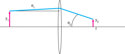
For a lens of focal length f illuminated by a beam of radius y1, the converging half-angle is approximately θ2 = y1/f. Applying the invariant gives the focused radius:
y2 = fθ1.
Consider the historical Newport R-31005 HeNe example: beam diameter 0.63 mm and full divergence 1.3 mrad, focused by a KPX043 lens with f = 25.4 mm. The inputs to the radius/half-angle calculation are y1 = 0.315 mm and θ1 = 0.65 mrad = 0.00065 rad.
y2 = (25.4 mm)(0.00065) = 0.01651 mm = 16.5 µm. The focused diameter is approximately 33 µm.
Within this model, replacing an already ideal lens with another lens of the same focal length cannot remove the incident beam’s angular spread. A shorter focal length reduces the calculated spot, while expanding the incident beam can reduce its divergence before focusing. Diffraction and aberrations can prevent the real spot from reaching the geometrical estimate.
2. Collimate light from a finite source or fiber
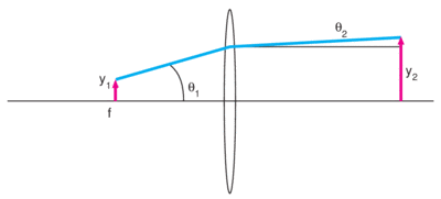
A source placed at the front focal plane produces a nominally collimated beam. A finite source radius y1 leaves a residual angular spread; it cannot become a perfect point source through choice of lens. If the collected input half-angle is θ1:
y2 ≈ fθ1; θ2 ≈ y1/f.
For the historical Newport F-MBB fiber example, the core diameter is 200 µm and the numerical aperture is 0.37. The source radius is therefore 100 µm = 0.1 mm. Using the source’s paraxial approximation θ1 ≈ NA = 0.37 in air and f = 25.4 mm gives:
- Beam radius: (25.4 mm)(0.37) ≈ 9.4 mm.
- Residual half-angle: 0.1 mm / 25.4 mm ≈ 3.94 mrad, rounded to 4 mrad.
Strictly, NA = n sin θ, so the equality between angle and NA is a small-angle approximation, with θ = arcsin(0.37) in air for the exact cone half-angle. At this aperture the approximation is useful for the source example, but an actual lens should be checked with its clear aperture and a nonparaxial ray model.
Doubling the focal length halves the residual divergence while doubling the beam radius in this model. Reducing beam diameter instead requires accepting greater angular spread. This tradeoff is central to long-distance collimation.
3. Build a Galilean beam expander
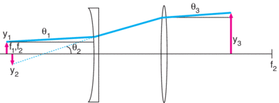
A Galilean expander uses a negative first lens and a positive second lens. Let their signed focal lengths be f1 < 0 and f2 > 0. For an afocal thin-lens arrangement, the separation is f1 + f2 = f2 − |f1|. The magnification is:
M = y3/y1 = f2/|f1|
2y3 = 2y1M; θ3 = θ1/M.
The negative lens creates a virtual source with radius approximately θ1|f1|. The positive lens recollimates that source. A fivefold expansion therefore reduces the ideal divergence by a factor of five; a tenfold expansion reduces it by ten.
Tenfold expansion example
Use the same 0.63 mm diameter, 1.3 mrad full-divergence HeNe beam with the historical Newport KPC043 negative lens, f1 = −25 mm, and KPX109 positive lens, f2 = 250 mm. The focal-length ratio is 10.
- Expanded diameter: (0.63 mm)(250/25) = 6.3 mm.
- Expanded half-angle divergence: (0.65 mrad)(25/250) = 0.065 mrad.
- The corresponding full divergence is 0.13 mrad.
- Thin-lens spacing: −25 mm + 250 mm = 225 mm.
Real lens surfaces and principal planes change the mechanical separation. The source example gives back focal lengths of −26.64 mm and 247.61 mm, whose sum is 220.97 mm. That number belongs to those particular lens prescriptions and spacing references; it should not be used for every −25 mm / 250 mm pair.
For the plano-concave/plano-convex pairing, orienting the plane faces toward one another helps control aberrations in this arrangement. Illuminating a central part of sufficiently large optics also reduces edge-ray aberrations and clipping. A Keplerian expander uses two positive lenses; for the same focal lengths its afocal separation is their positive sum and it includes an internal real focus.
4. Image an extended source onto a small spot
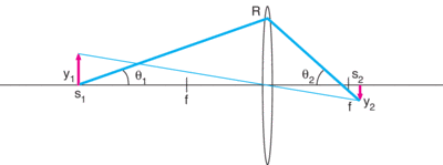
Imaging a fluorescent sample onto a camera is an extended-source problem. Let the source radius be y1, object distance s1, image distance s2, and lens clear radius R. The thin-lens equation is 1/f = 1/s1 + 1/s2. For a distant object, s2 is close to f.
With θ1 ≈ R/s1 and θ2 ≈ R/f, the invariant gives:
y2 ≈ y1f/s1 = 2y1(R/s1)(F/#), where F/# = f/(2R).
Image magnification is principally determined by the conjugate distances and focal length. Stopping down a fixed lens changes R and F/# in opposite directions, leaving the ideal geometrical image size unchanged; it reduces collected power. Halving the aperture radius reduces the small-angle collection solid angle by about four. Doubling the source distance also reduces that solid angle by about four, and for a distant source reduces the image magnification by about two.
A shorter focal length at the same aperture can make the geometrical image smaller, but a very fast lens brings stronger aberration and acceptance constraints. The source’s suggestion of F/1 as a practical boundary is an application-dependent guideline, not a universal optical limit. Evaluate image size, captured light and actual image quality together.